Evaluating Trading Strategy: A Comprehensive Guide to Performance Comparison

In the world of financial markets, the ability to assess and compare the performance of different trading strategies is crucial for success. Traders and investors need to ensure that the strategies they employ not only generate profits but also outperform alternative methods consistently. This is where the evaluation of strategy performance and comparability becomes invaluable.

For more information on Monte Carlo Simulations, visit QuantEdX

Why Should We Evaluate Trading Strategy Performance?

Evaluating the performance of trading strategies is essential for several reasons:

1. Profit Maximization: The primary objective of any trading strategy is to maximize profits. By comparing strategies, traders can identify which ones have the potential to yield higher returns.
2. Risk Management: Understanding the risk associated with each strategy is critical. Some strategies may deliver higher returns but come with greater risk, while others may be more conservative. Comparing strategies helps strike the right balance between risk and reward.
3. Benchmarking: Traders often compare their strategies against benchmark indices or other well-established standards to assess their relative performance. This ensures that a strategy is competitive within its market.
4. Adaptation: Markets are dynamic, and strategies that once performed well may become less effective over time. Regular evaluation allows traders to adapt and refine their approaches to changing market conditions.

Let’s dive into a step-by-step guide to evaluate and compare trading strategies, complete with Python code examples:

Step 1: Data Import and Trading Strategy Implementation

To begin, import historical financial data from a reliable source such as Yahoo Finance. For demonstration purposes, we’ll use two popular trading strategies: Simple Moving Average (SMA) Crossover and Moving Average Convergence Divergence (MACD) with Relative Strength Index (RSI).

import pandas as pd
import yfinance as yf
import matplotlib.pyplot as plt
from scipy.stats import ttest_rel

# Define the tickers and download data from Yahoo Finance
tickers = ["AAPL", "MSFT"]
start_date = "2010-01-01"
end_date = "2021-12-31"

data = yf.download(tickers, start=start_date, end=end_date)["Adj Close"]

Step 2: Calculate Cumulative Returns

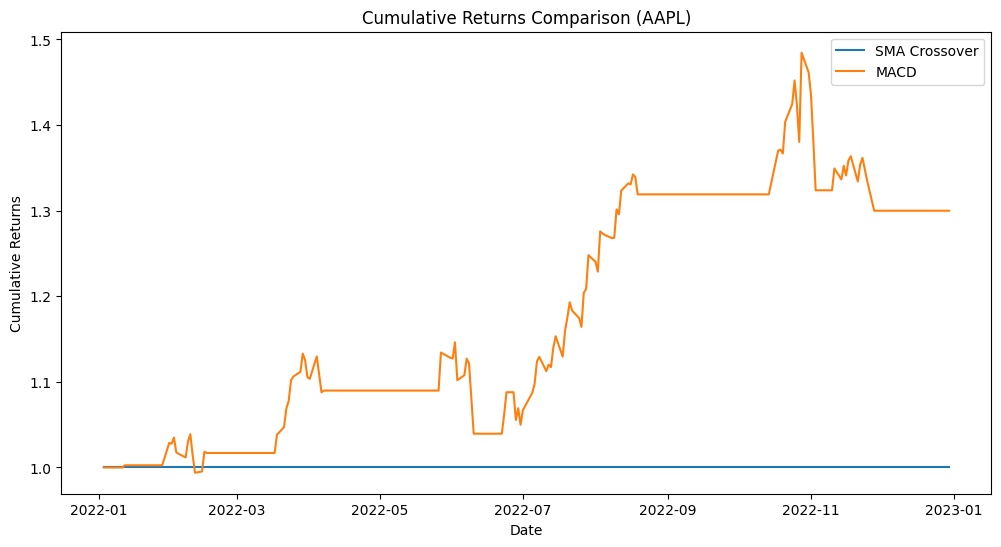
Calculate the cumulative returns of each strategy over the specified time frame. Cumulative returns provide a clear picture of how the strategies perform over time.

# Calculate SMA Crossover strategy returns
sma_short_window = 50
sma_long_window = 200

sma_short = data.rolling(window=sma_short_window).mean()
sma_long = data.rolling(window=sma_long_window).mean()

sma_strategy_returns = (sma_long.shift(-1) > sma_short.shift(-1)) * data.pct_change()

# Calculate MACD with RSI strategy returns
short_window = 12
long_window = 26
signal_window = 9

ema_short = data.ewm(span=short_window, adjust=False).mean()
ema_long = data.ewm(span=long_window, adjust=False).mean()

macd = ema_short - ema_long
signal = macd.rolling(window=signal_window).mean()

rsi_window = 14
delta = data.diff()
gain = (delta.where(delta > 0, 0)).fillna(0)
loss = (-delta.where(delta < 0, 0)).fillna(0)

average_gain = gain.rolling(window=rsi_window).mean()
average_loss = loss.rolling(window=rsi_window).mean()
rs = average_gain / average_loss
rsi = 100 - (100 / (1 + rs))

macd_rsi_strategy_returns = ((macd.shift(-1) > signal.shift(-1)) & (rsi.shift(-1) > 70)) * data.pct_change()

# Calculate cumulative returns
sma_cumulative_returns = (1 + sma_strategy_returns).cumprod()
macd_rsi_cumulative_returns = (1 + macd_rsi_strategy_returns).cumprod()

# Plot cumulative returns
plt.figure(figsize=(12, 6))
plt.plot(sma_cumulative_returns, label="SMA Crossover")
plt.plot(macd_rsi_cumulative_returns, label="MACD with RSI")
plt.legend()
plt.title("Cumulative Returns of SMA Crossover vs. MACD with RSI Strategies")
plt.xlabel("Date")
plt.ylabel("Cumulative Return")
plt.show()

Step 3: Perform a T-Test on Trading Strategy Returns

Now, assess the significance of any performance differences between the strategies using a T-test. The T-test helps determine if the differences in returns are statistically significant or merely due to chance.

# Perform a T-test to assess the significance of the improvement
t_statistic, p_value = ttest_rel(sma_strategy_returns.fillna(0), macd_rsi_strategy_returns.fillna(0), nan_policy='omit')

# Evaluate the results
if p_value < 0.05:  # Significance level of 5%
    print("The improvement in the MACD with RSI strategy is statistically significant.")
else:
    print("The improvement in the MACD with RSI strategy is not statistically significant.")

Step 4: Monte Carlo Simulation to evaluate performance

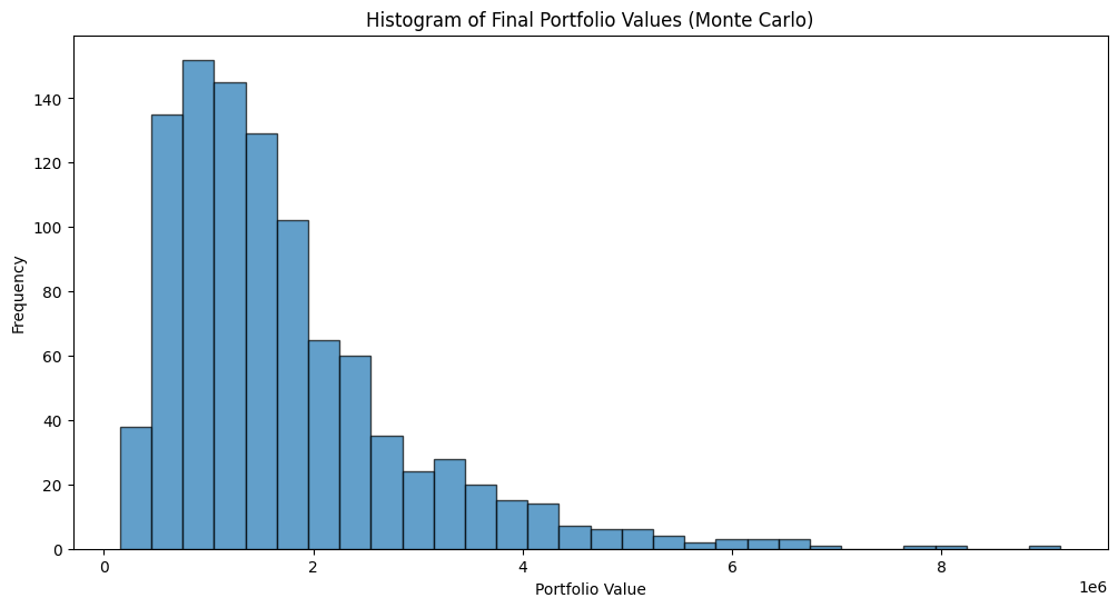
For a more robust assessment, apply a Monte Carlo simulation. This technique involves generating numerous random alternative scenarios based on historical data. By comparing the actual strategy performance with these simulations, you gain insights into the strategy’s robustness.

# Define parameters for the Monte Carlo simulation
num_simulations = 1000  # Number of simulation runs
simulation_years = 5    # Number of years to simulate
initial_portfolio_value = 100000  # Initial portfolio value in dollars

# Calculate daily returns for the selected trading strategy (e.g., SMA Crossover)
# Replace this with the actual daily returns of your strategy
strategy_daily_returns = np.random.normal(0.0005, 0.02, (simulation_years * 252,))

# Perform the Monte Carlo simulation
final_portfolio_values = []

for _ in range(num_simulations):
    portfolio_value = initial_portfolio_value
    for _ in range(simulation_years * 252):
        # Simulate daily returns
        daily_return = np.random.choice(strategy_daily_returns)
        # Update portfolio value
        portfolio_value *= (1 + daily_return)
    final_portfolio_values.append(portfolio_value)

# Calculate statistics from the simulation results
mean_final_portfolio_value = np.mean(final_portfolio_values)
std_final_portfolio_value = np.std(final_portfolio_values)
percentile_10th = np.percentile(final_portfolio_values, 10)
percentile_90th = np.percentile(final_portfolio_values, 90)

# Print simulation results
print("Monte Carlo Simulation Results:")
print(f"Mean Final Portfolio Value: ${mean_final_portfolio_value:.2f}")
print(f"Standard Deviation of Final Portfolio Value: ${std_final_portfolio_value:.2f}")
print(f"10th Percentile Final Portfolio Value: ${percentile_10th:.2f}")
print(f"90th Percentile Final Portfolio Value: ${percentile_90th:.2f}")

Step 5: Bootstrap Analysis for Trading Strategy Returns

Bootstrap analysis complements the Monte Carlo simulation by resampling data with replacement to estimate the distribution of returns. This helps evaluate the probability of achieving the observed strategy performance by chance.

For more such trading Strategies, visit us at Quantified Trader/Trading Strategies

What is t – test?

A t-test, also known as a Student’s t-test, is a statistical hypothesis test used to determine if there is a significant difference between the means of two groups or sets of data. It helps in comparing the averages (means) of two samples to assess whether any observed differences are statistically significant or simply due to random chance.

There are different types of t-tests, but the most common ones include:

1. Independent Samples t-test: This type of t-test is used when you want to compare the means of two separate and unrelated groups or populations. For example, you might use it to compare the average test scores of two different classes of students to see if one class performed significantly better than the other.
2. Paired Samples t-test: This t-test is used when you want to compare the means of two related groups, often before and after an intervention or treatment. For instance, you might use it to determine if a new teaching method significantly improved students’ test scores compared to their scores before the new method was implemented.

The t-test generates a t-statistic and a p-value as part of its output. The t-statistic quantifies the difference between the sample means and takes into account the sample sizes and standard deviations. The p-value indicates the probability of obtaining such results by random chance if there is no real difference between the groups.

In hypothesis testing, you typically set a significance level (alpha), often at 0.05 (5%), which represents the threshold below which you consider the results to be statistically significant. If the p-value calculated by the t-test is less than the significance level (usually 0.05), you reject the null hypothesis (which assumes no difference) in favor of the alternative hypothesis, suggesting that there is a significant difference between the groups.

In summary, a t-test is a statistical tool used to determine if the differences between two sets of data are likely due to a real effect or if they could have occurred by random chance. It is widely used in various fields, including science, medicine, economics, and social sciences, for comparing means and drawing conclusions about the significance of observed differences.

Conclusion

Evaluating and comparing trading strategies is a critical aspect of successful trading and investment. It ensures that strategies are not only profitable but also resilient to market variations. By following a systematic approach that includes data analysis, statistical tests like the T-test, and simulation techniques like Monte Carlo and bootstrap analysis, traders and investors can make informed decisions and enhance their chances of success in the dynamic world of financial markets.